 Deep Learning of MNIST handwritten digits
In this document I am going create a video showing the training of the inner-most layer of Deep Belief Network (DBN) using the MNIST dataset of handwritten digits. I will use our DeepLearning R package that implements flexible DBN architectures with an object-oriented interface.
MNIST
The MNIST dataset is a database of handwritten digits with 60,000 training images and 10,000 testing images. You can learn everything about it on Wikipedia. In short, it is the go-to dataset to train and test handwritten digit recognition machine learning algorithms.
I made an R package for easy access, named mnist. The easiest way to install it is with devtools. If you don't have it already, let's first install devtools:
if (!require("devtools")) {install.packages("devtools")}
Now we can install mnist:
devtools::install_github("xrobin/mnist")
PCA
In order to see what the dataset looks like, let's use PCA to reduce it to two dimensions.
pca <- prcomp(mnist$train$x)
plot.mnist(
	prediction = predict(pca, mnist$test$x),
	reconstruction = tcrossprod(
		predict(pca, mnist$test$x)[,1:2], pca$rotation[,1:2]),
	highlight.digits = c(72, 3, 83, 91, 6688, 7860, 92, 1, 180, 13))
Let's take a minute to describe this plot. The central scatterplot shows first two components of the PCA of all digits in the test set. On the left hand side, I picked 10 representative digits from the test set to highlight, which are shown as larger circles in the central scatterplot. On the left are the "reconstructed digits", which were reconstructed from the two first dimensions of the PCA. While we can see some digit-like structures, it is basically impossible to recognize them. We can see some separation of the digits in the 2D space as well, but it is pretty weak and some pairs cannot be distinguished at all (like 4 and 9). Of course the reconstructions would look much better had we kept all PCA dimensions, but so much for dimensionality reduction.
Deep Learning
Now let's see if we can do better with Deep Learning. We'll use a classical Deep Belief Network (DBN), based on Restricted Boltzmann Machines (RBM) similar to what Hinton described back in 2006 (Hinton & Salakhutdinov, 2006). The training happens in two steps: a pre-training step with contrastive divergence stochastic gradient descent brings the network to a reasonable starting point for a more conventional conjugate gradient optimization (hereafter referred to as fine-tuning).
I implemented this algorithm with a few modifications in an R package which is available on GitHub. The core of the processing is done in C++ with RcppEigen (Bates & Eddelbuettel, 2013) for higher speed. Using devtools again:
devtools::install_github("xrobin/DeepLearning")
We will use this code to train a 5 layers deep network, that reduces the digits to an abstract, 2D representation. By looking at this last layer throughout the training process we can start to understand how the network learns to recognize digits. Let's start by loading the required packages and the MNIST dataset, and create the DBN.
library(DeepLearning)
library(mnist)
data(mnist)

dbn <- DeepBeliefNet(Layers(c(784, 1000, 500, 250, 2),
	input = "continuous", output = "gaussian"),
	initialize = "0")
We just created the 5-layers DBN, with continuous, 784 nodes input (the digit image pixels), and a 2 nodes, gaussian output. It is initialized with 0, but we could have left out the initialize to start from a random initilization (Bengio et al., 2007). Before we go, let's define a few useful variables:
output.folder <- "video" # Where to save the output
maxiters.pretrain <- 1e6  # Number of pre-training iterations
maxiters.train <- 10000 # Number of fine-tuning iterations
run.training <- run.images <- TRUE # Turn any of these off
# Which digits to highlight and reconstruct
highlight.digits = c(72, 3, 83, 91, 6688, 7860, 92, 1, 180, 13)
We'll also need the following function to show the elapsed time:
format.timediff <- function(start.time) {
    diff = as.numeric(difftime(Sys.time(), start.time, units="mins"))
    hr <- diff%/%60
    min <- floor(diff - hr * 60)
    sec <- round(diff%%1 * 60,digits=2)
    return(paste(hr,min,sec,sep=':'))
}
Pre-training
Initially, the network is a stack of RBMs that we need to pre-train one by one. Hinton & Salakhutdinov (2006) showed that this step is critical to train deep networks. We will use 1000000 iterations (maxiters.pretrain) of contrastive divergence, which takes a couple of days on a modern CPU. Let's start with the first three RBMs:
First three RBMs
if (run.training) {
	sprintf.fmt.iter <- sprintf("%%0%dd", nchar(sprintf("%d", maxiters.pretrain)))

	mnist.data.layer <- mnist
	for (i in 1:3) {
We define a diag function that will simply print where we are in the training. Because this function will be called a million times (maxiters.pretrain), we can use rate = "accelerate" to slow down the printing over time and save a few CPU cycles.
		diag <- list(rate = "accelerate", data = NULL, f = function(rbm, batch, data, iter, batchsize, maxiters, layer) {
			print(sprintf("%s[%s/%s] in %s", layer, iter, maxiters, format.timediff(start.time)))
		})
We can get the current RBM, and we will work on it directly. Let's save it for good measure, as well as the current time for the progress function:
		rbm <- dbn[[i]]
		save(rbm, file = file.path(output.folder, sprintf("rbm-%s-%s.RData", i, "initial")))
		start.time <- Sys.time()
Now we can start the actual pre-training:
		rbm <- pretrain(rbm, mnist.data.layer$train$x,
			penalization = "l2", lambda=0.0002, momentum = c(0.5, 0.9),
			epsilon=c(.1, .1, .1, .001)[i], batchsize = 100, maxiters=maxiters.pretrain,
			continue.function = continue.function.always, diag = diag)
This can take some time, especially for the first layers which are larger. Once it is done, we predict the data through this RBM for the next layer and save the results:
		mnist.data.layer$train$x <- predict(rbm, mnist.data.layer$train$x)
		mnist.data.layer$test$x <- predict(rbm, mnist.data.layer$test$x)
		save(rbm, file = file.path(output.folder, sprintf("rbm-%s-%s.RData", i, "final")))
		dbn[[i]] <- rbm
	}
Last RBM
This is very similar to the previous three, but note that we save the RBM within the diag function. We could generate the plot directly, but it is easier to do it later once we have some idea about the final axis we will need. Please note the rate = "accelerate" here. You probably don't want to save a million RBM objects on your hard drive, both for speed and space reasons.
	rbm <- dbn[[4]]
	print(head(rbm$b))
	diag <- list(rate = "accelerate", data = NULL, f = function(rbm, batch, data, iter, batchsize, maxiters, layer) {
		save(rbm, file = file.path(output.folder, sprintf("rbm-4-%s.RData", sprintf(sprintf.fmt.iter, iter))))
		print(sprintf("%s[%s/%s] in %s", layer, iter, maxiters, format.timediff(start.time)))
	})
	save(rbm, file = file.path(output.folder, sprintf("rbm-%s-%s.RData", 4, "initial")))
	start.time <- Sys.time()
	rbm <- pretrain(rbm, mnist.data.layer$train$x,  penalization = "l2", lambda=0.0002,
		epsilon=.001, batchsize = 100, maxiters=maxiters.pretrain,
		continue.function = continue.function.always, diag = diag)
	save(rbm, file = file.path(output.folder, sprintf("rbm-4-%s.RData", "final")))
	dbn[[4]] <- rbm
If we were not querying the last layer, we could have pre-trained the entire network at once with the following call:
	dbn <- pretrain(dbn, mnist.data.layer$train$x,
		penalization = "l2", lambda=0.0002, momentum = c(0.5, 0.9),
		epsilon=c(.1, .1, .1, .001), batchsize = 100,
		maxiters=maxiters.pretrain,
		continue.function = continue.function.always)
Pre-training parameters
Pre-training RBMs is quite sensitive to the use of proper parameters. With improper parameters, the network can quickly go crazy and start to generate infinite values. If that happens to you, you should try to tune one of the following parameters:
penalization: this is the penalty of introducing or increasing the value of a weight. We used L2 regularization, but"l1"is available if a sparser weight matrix is needed.lambda: the regularization rate. In our experience 0.0002 works fine with the MNIST and other datasets of similar sizes such as cellular imaging data. Too small or large values will result in over- or under-fitted networks, respectively.momentum: helps avoiding oscillatory behaviors, where the network oscillate between iterations. Allowed values can range from 0 (no momentum) to 1 (full momentum = no training). Here we used an increasing gradient of momentum which starts at 0.5 and increases linearly to 0.9, in order to stabilize the final network without compromising early training steps.epsilon: the learning rate. Typically, 0.1 works well with binary and continuous output layers, and must be decreased to around 0.001 for gaussian outputs. Too large values will drive the network to generate infinities, while too small ones will slow down the training.batchsize: larger batch sizes will result in smoother but slower training. Small batch sizes will make the training "jumpy", which can be compensated by lower learning rates (epsilon) or increased momentum.
Fine-tuning
This is where the real training happens. We use conjugate gradients to find the optimal solution. Again, the diag function saves the DBN. This time we use rate = "each" to save every step of the training. First we have way fewer steps, but also the training itself happen at a much more stable speed than in the pre-training, where things slow down dramatically.
	sprintf.fmt.iter <- sprintf("%%0%dd", nchar(sprintf("%d", maxiters.train)))
	diag <- list(rate = "each", data = NULL, f = function(dbn, batch, data, iter, batchsize, maxiters) {
		save(dbn, file = file.path(output.folder, sprintf("dbn-finetune-%s.RData", sprintf(sprintf.fmt.iter, iter))))
		print(sprintf("[%s/%s] in %s", iter, maxiters, format.timediff(start.time)))
	})
	save(dbn, file = file.path(output.folder, sprintf("dbn-finetune-%s.RData", "initial")))
	start.time <- Sys.time()
	dbn <- train(unroll(dbn), mnist$train$x, batchsize = 100, maxiters=maxiters.train,
		continue.function = continue.function.always, diag = diag)
	save(dbn, file = file.path(output.folder, sprintf("dbn-finetune-%s.RData", "final")))
}
And that's it, our DBN is now fully trained!
Generating the images
Now we need to read in the saved network states again, pass the data through the network (predict) and save this in HD-sized PNG file.
The first three RBMs are only loaded into the DBN
if (run.images) {
	for (i in 1:3) {
		load(file.path(output.folder, sprintf("rbm-%d-final.RData", i)))
		dbn[[i]] <- rbm
	}
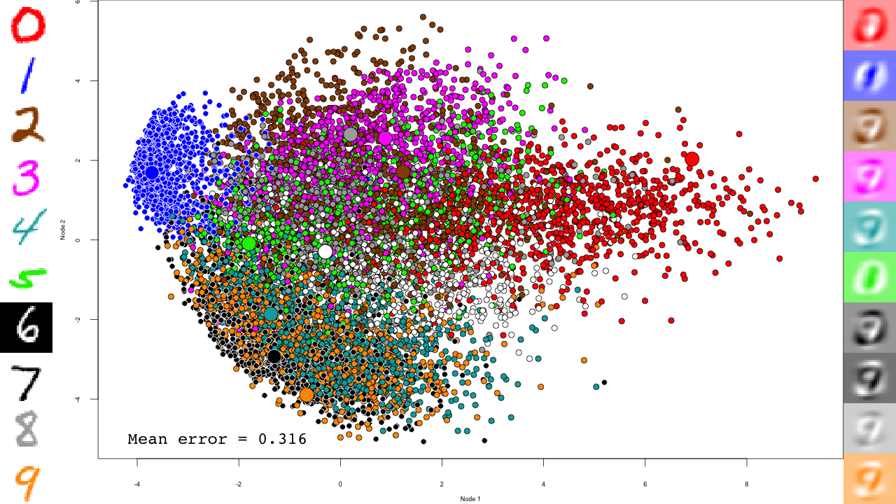
The last RBM is where interesting things happen.
	for (file in list.files(output.folder, pattern = "rbm-4-.+\\.RData", full.names = TRUE)) {
		print(file)
		load(file)
		dbn[[4]] <- rbm
		iter <- stringr::str_match(file, "rbm-4-(.+)\\.RData")[,2]
We now predict and reconstruct the data, and calculate the mean reconstruction error:
		predictions <- predict(dbn, mnist$test$x)
		reconstructions <- reconstruct(dbn, mnist$test$x)
		iteration.error <- errorSum(dbn, mnist$test$x) / nrow(mnist$test$x)
Now the actual plotting. Here I selected xlim and ylim values that worked well for my training run, but your mileage may vary.
		png(sub(".RData", ".png", file), width = 1280, height = 720) # hd output
		plot.mnist(model = dbn, x = mnist$test$x, label = mnist$test$y+1, predictions = predictions, reconstructions = reconstructions,
				   ncol = 16, highlight.digits = highlight.digits,
				   xlim = c(-12.625948, 8.329168), ylim = c(-10.50657, 13.12654))
		par(family="mono")
		legend("bottomleft", legend = sprintf("Mean error = %.3f", iteration.error), bty="n", cex=3)
		legend("bottomright", legend = sprintf("Iteration = %s", iter), bty="n", cex=3)
		dev.off()
	}
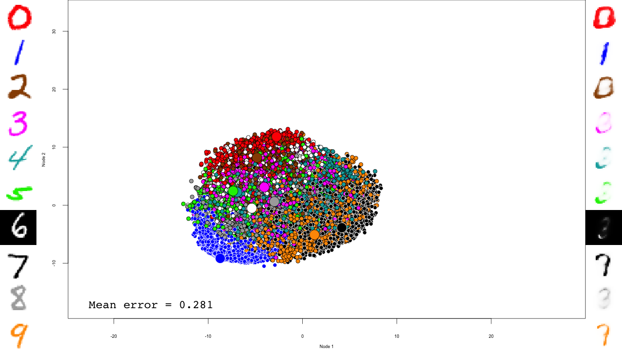
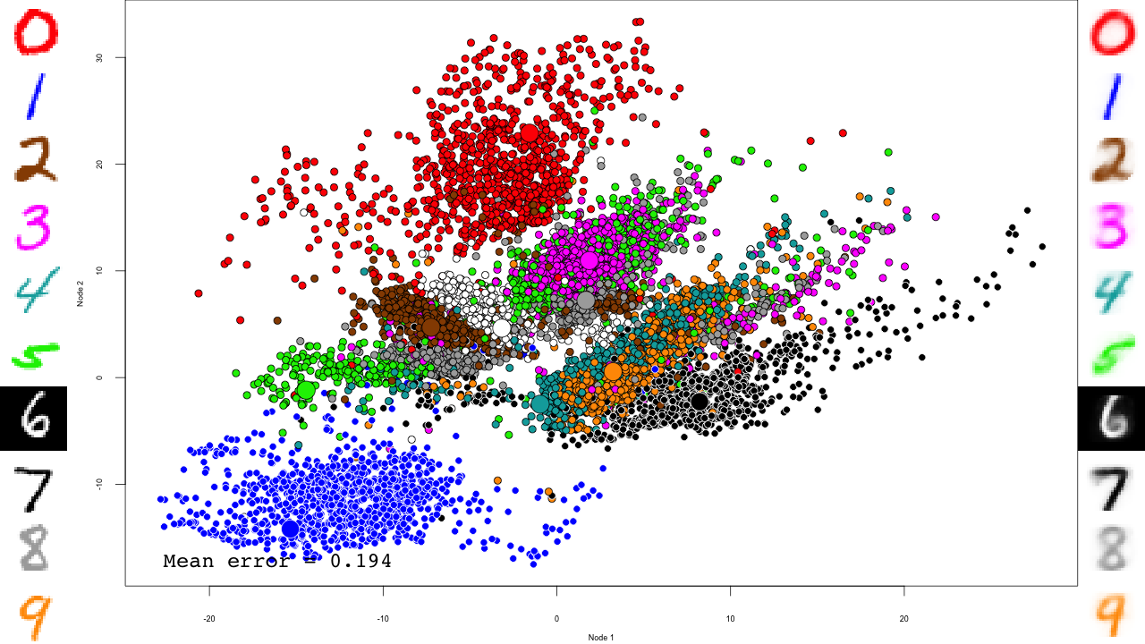
We do the same with the fine-tuning:
	for (file in list.files(output.folder, pattern = "dbn-finetune-.+\\.RData", full.names = TRUE)) {
		print(file)
		load(file)
		iter <- stringr::str_match(file, "dbn-finetune-(.+)\\.RData")[,2]
		predictions <- predict(dbn, mnist$test$x)
		reconstructions <- reconstruct(dbn, mnist$test$x)
		iteration.error <- errorSum(dbn, mnist$test$x) / nrow(mnist$test$x)
		png(sub(".RData", ".png", file), width = 1280, height = 720) # hd output
		plot.mnist(model = dbn, x = mnist$test$x, label = mnist$test$y+1, predictions = predictions, reconstructions = reconstructions,
				   ncol = 16, highlight.digits = highlight.digits,
				   xlim = c(-22.81098,  27.94829), ylim = c(-17.49874,  33.34688))
		par(family="mono")
		legend("bottomleft", legend = sprintf("Mean error = %.3f", iteration.error), bty="n", cex=3)
		legend("bottomright", legend = sprintf("Iteration = %s", iter), bty="n", cex=3)
		dev.off()
	}
}
The video
I simply used ffmpeg to convert the PNG files to a video:
cd video
ffmpeg -pattern_type glob -i "rbm-4-*.png" -b:v 10000000 -y ../rbm-4.mp4
ffmpeg -pattern_type glob -i "dbn-finetune-*.png" -b:v 10000000 -y ../dbn-finetune.mp4
And that's it! Notice how the pre-training only brings the network to a state similar to that of a PCA, and the fine-tuning actually does the separation, and how it really makes the reconstructions accurate.
Application
We used this code to analyze changes in cell morphology upon drug resistance in cancer. With a 27-dimension space, we could describe all of the observed cell morphologies and predict whether a cell was resistant to ErbB-family drugs with an accuracy of 74%. The paper is available in Open Access in Cell Reports, DOI 10.1016/j.celrep.2020.108657.
Concluding remarks
In this document I described how to build and train a DBN with the DeepLearning package. I also showed how to query the internal layer, and use the generative properties to follow the training of the network on handwritten digits.
DBNs have the advantage over Convolutional Networks (CN) that they are fully generative, at least during the pre-training. They are therefore easier to query and interpret as we have demonstrated here. However keep in mind that CNs have demonstrated higher accuracies on computer vision tasks, such as the MNIST dataset.
Additional algorithmic details are available in the doc folder of the DeepLearning package.
References
- Our paper, 2021
- Longden J., Robin X., Engel M., et al. Deep neural networks identify signaling mechanisms of ErbB-family drug resistance from a continuous cell morphology space. Cell Reports, 2021;34(3):108657.
- Bates & Eddelbuettel, 2013
- Bates D, Eddelbuettel D. Fast and Elegant Numerical Linear Algebra Using the RcppEigen Package. Journal of Statistical Software, 2013;52(5):1–24.
- Bengio et al., 2007
- Bengio Y, Lamblin P, Popovici D, Larochelle H. Greedy layer-wise training of deep networks. Advances in neural information processing systems. 2007;19:153–60.
- Hinton & Salakhutdinov, 2006
- Hinton GE, Salakhutdinov RR. Reducing the Dimensionality of Data with Neural Networks. Science. 2006;313(5786):504–7.
Downloads
Xavier Robin
Published Saturday, June 11, 2022 16:39 CEST
Permalink: /blog/2022/06/11/deep-learning-of-mnist-handwritten-digits
Tags:
Programming
Comments: 0
 Search
 Tags
Tags Recent posts
 Calendar
 Syndication